From R-Scripts to Katonic Pipeline using Katonic Studio
1. Get Started
Jupyter Notebook is a very popular tool that data scientists use every day to write their ML code, experiments, and visualize the results. However, when it comes to converting a Notebook to a Pipeline, data scientists struggle a lot. It is a very challenging, time-consuming task, and most of the time it needs the cooperation of several different subject-matter experts: Data Scientist, Machine Learning Engineer, Data Engineer.
A typical machine/deep learning pipeline begins as a series of preprocessing steps followed by experimentation/optimization and finally deployment. Each of these steps represents a challenge in the model development lifecycle. Katonic Studio provides a Pipeline Visual Editor for building AI pipelines from notebooks, Python scripts and R scripts, simplifying the conversion of multiple notebooks or scripts files into batch jobs or workflows.
This tutorial will guide you to use the Katonic Studio to assemble pipelines from R notebooks or scripts without the need for any coding.
1.1 Sign In
Once the admin creates your ID in the respective cluster, you will get your username and temporary password over the e-mail.
Open the login page,set your permanent password and login to try the Katonic platform.

Enter your email and password, and click on the “Sign In” button to sign in to the platform.
1.2 Orient yourself to the Katonic platform
When you first log in, you will find yourself in the Dashboard section of Katonic. You can use the left sidebar to navigate to other sections of Katonic Platform.
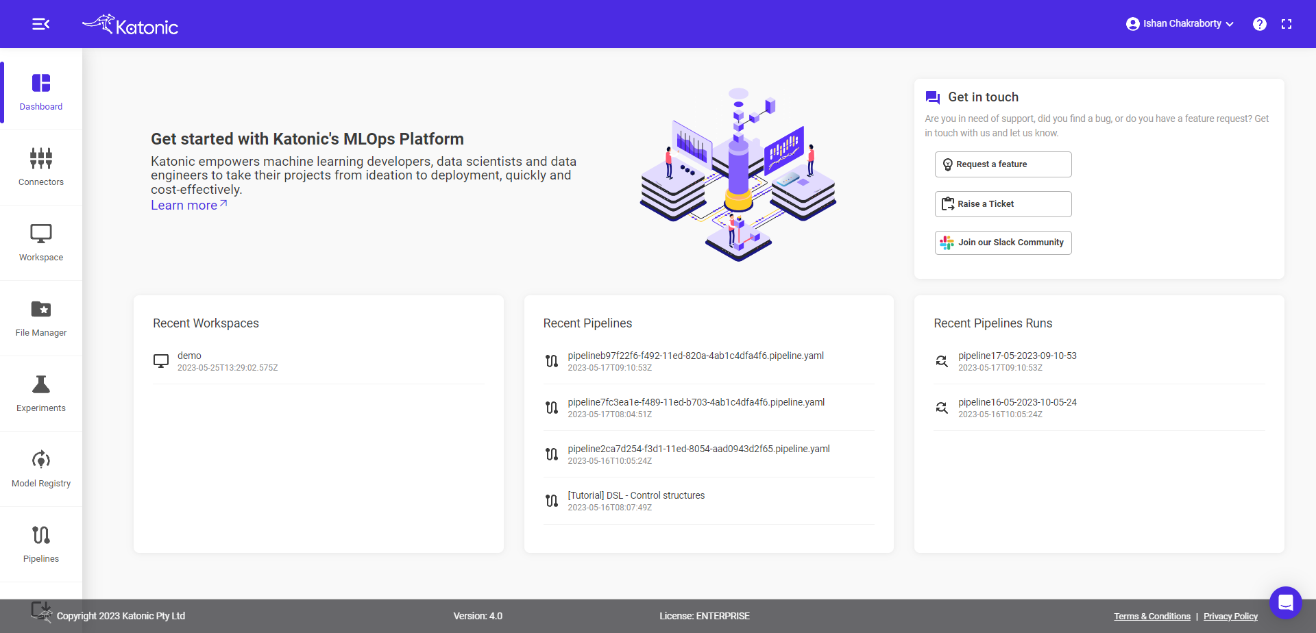
To view the platform in full screen click on the “full-screen mode“ on the top right of the page.
If you would like to search the Katonic documentation for help, click on the “?” icon on the top right of the page.
To send a question to a member of the Katonic support staff, use the Support button on the bottom right of the page.
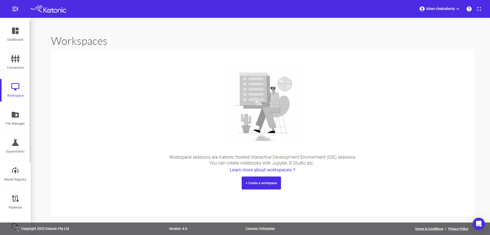
1.3 Create a Workspace
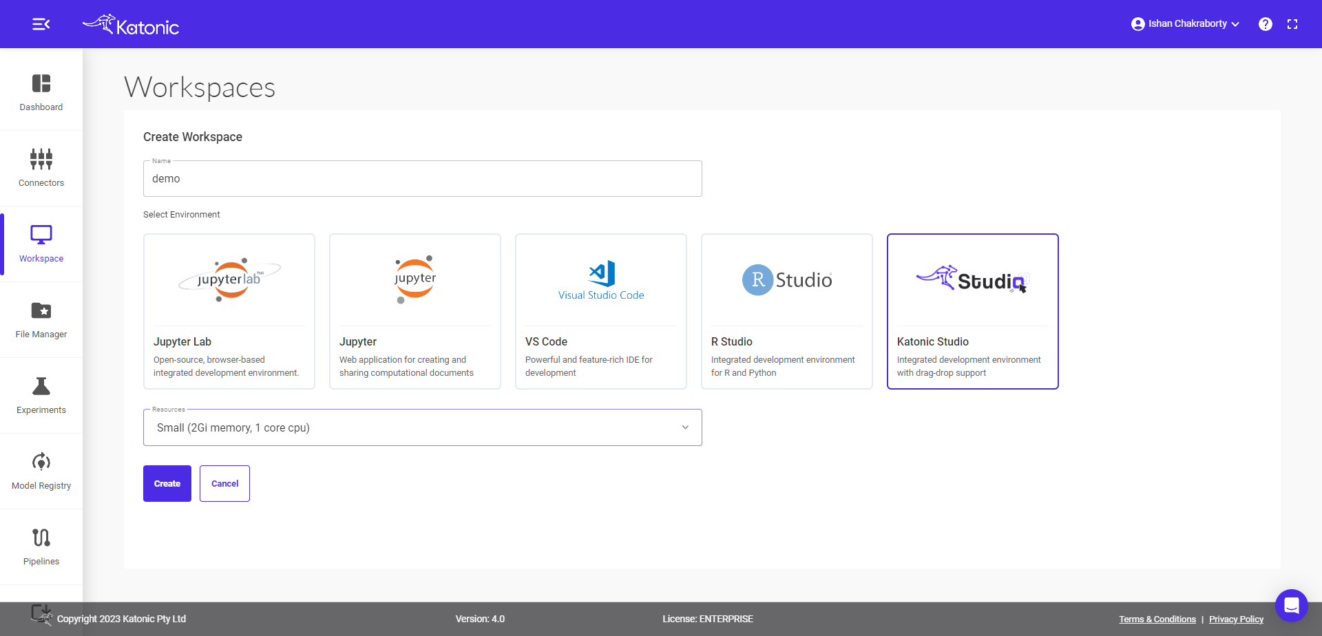
From the Workspace on the left panel, Click on ‘Create Workspace’ in the top right side of the page.
Fill in the following details.
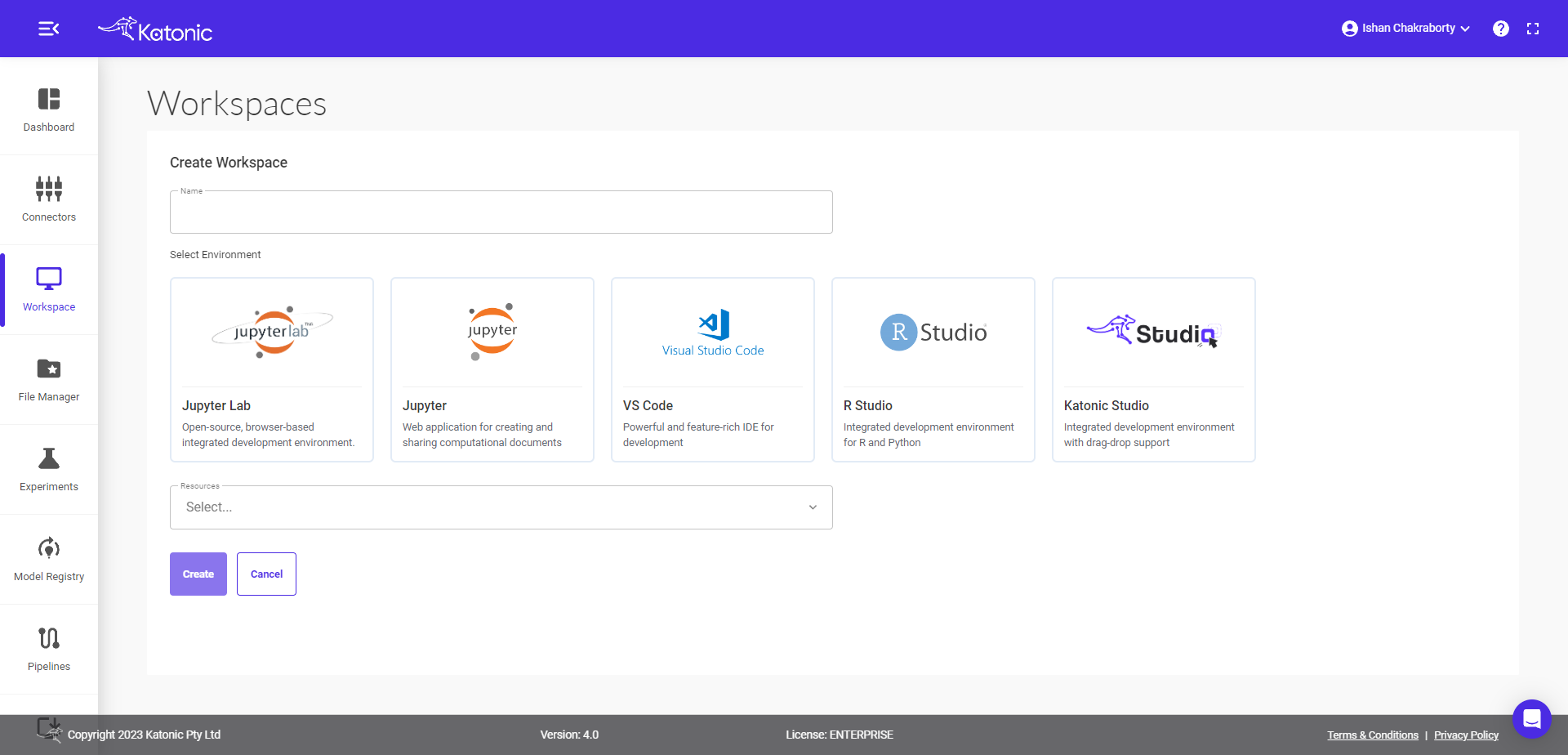
Give your Workspace an informative name (like amazon-revenue).
Note : Workspace name should contain only lowercase(a-z), numbers(0-9) and hyphen(-).
Select Environment as Katonic Studio.
Select the Number of CPUs and the memory you want to allocate to Workspace.
click on Create.
1.4 Start Workspace
Once you create a workspace you could see it will be in 'processing' state.
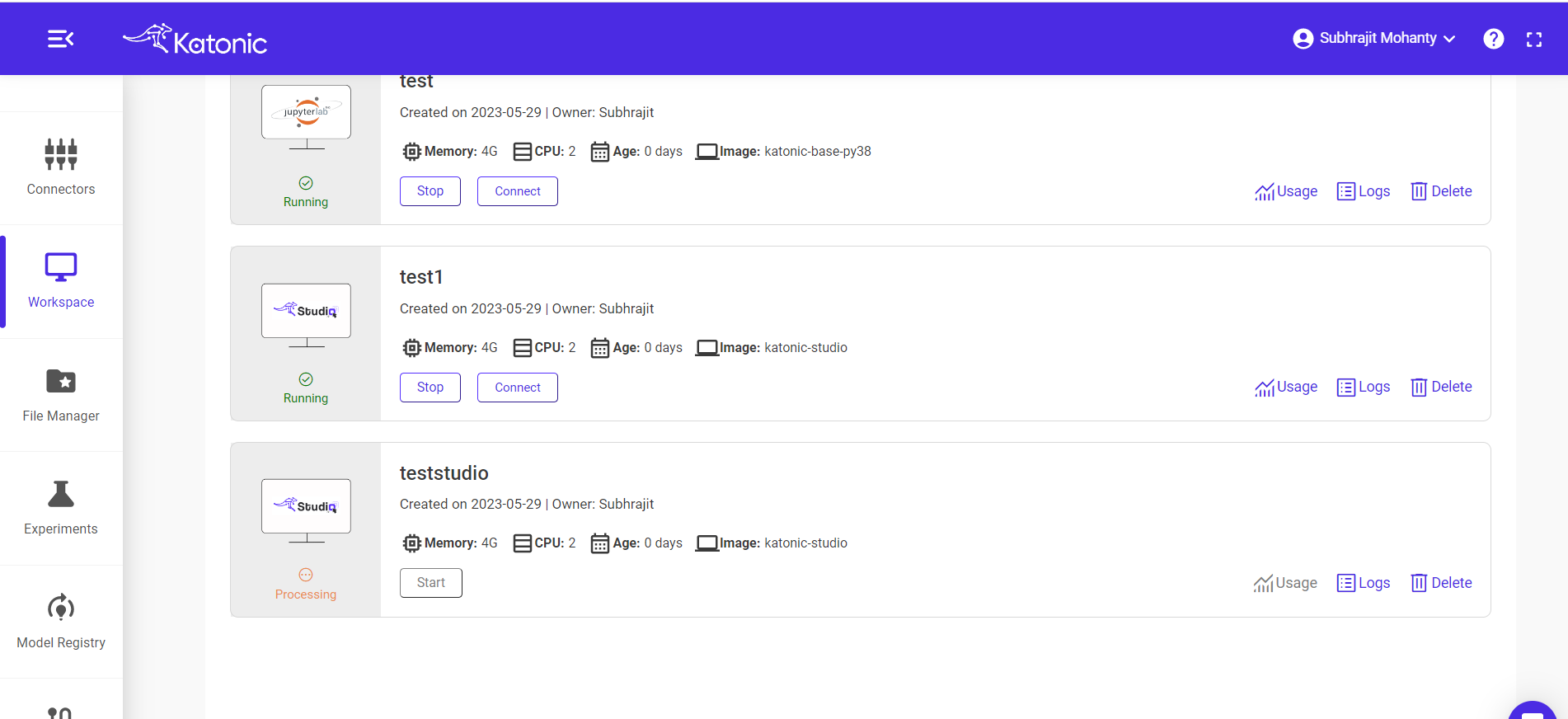
Once the workspace has started it will show the connect button with which you can connect to the notebook server.
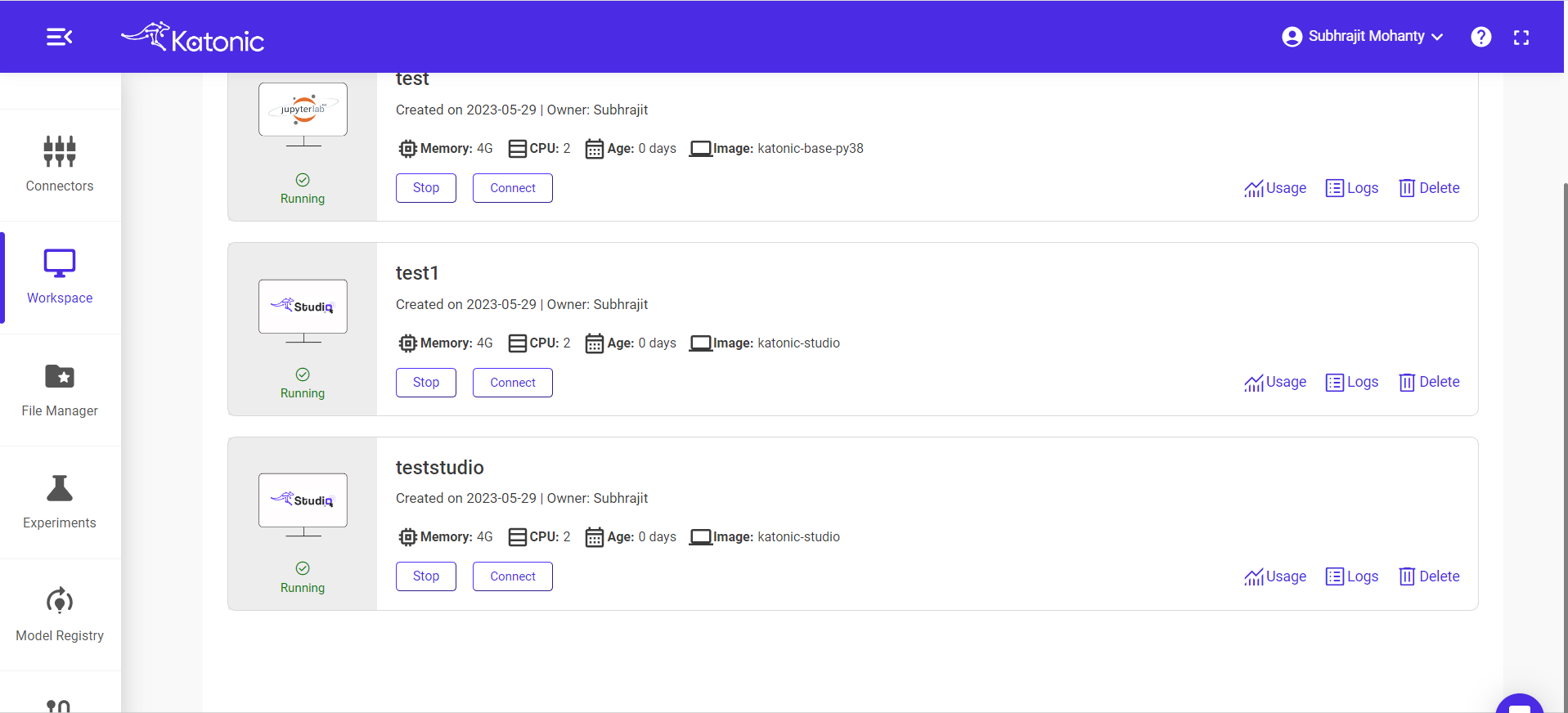
When you connect a workspace, a new session is created on a machine and your browser is automatically redirected to the notebook UI.
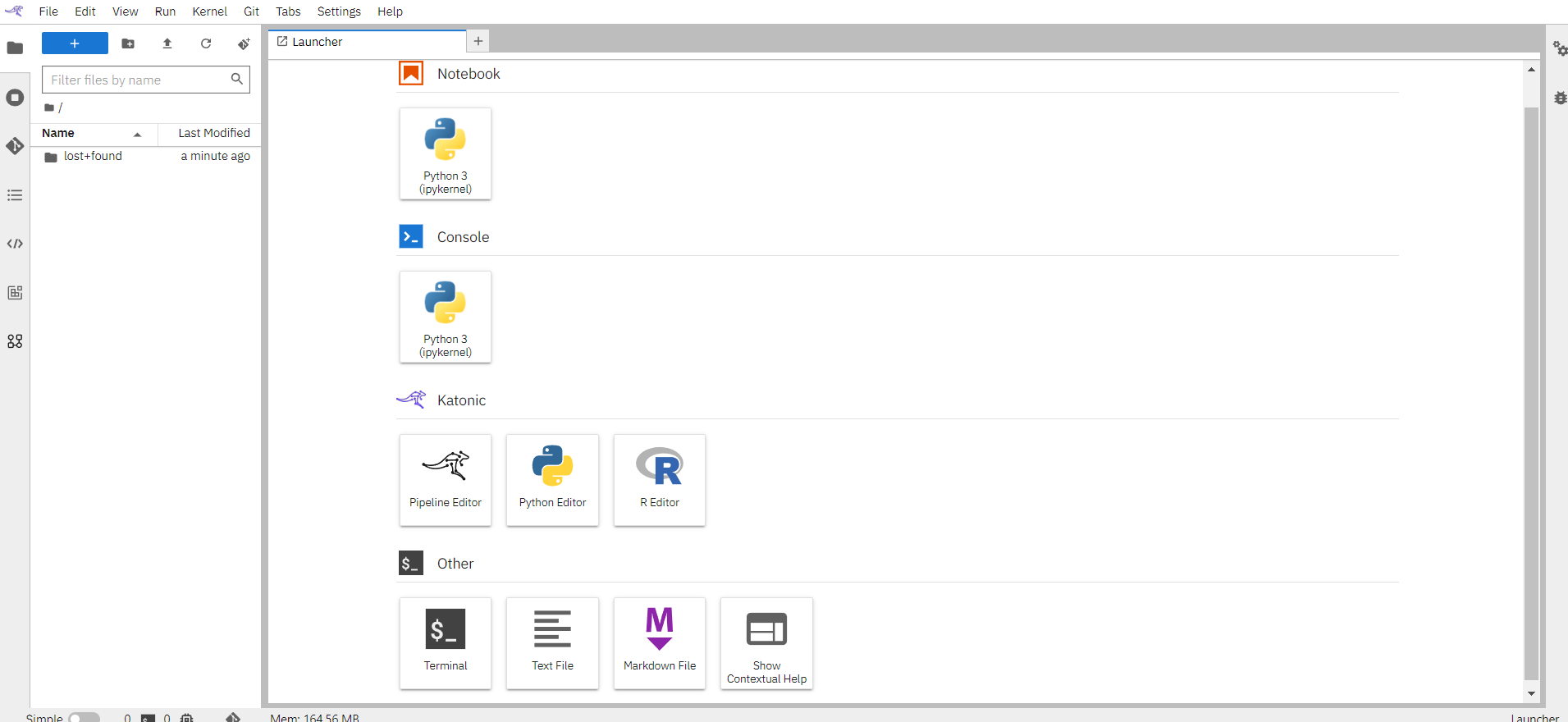
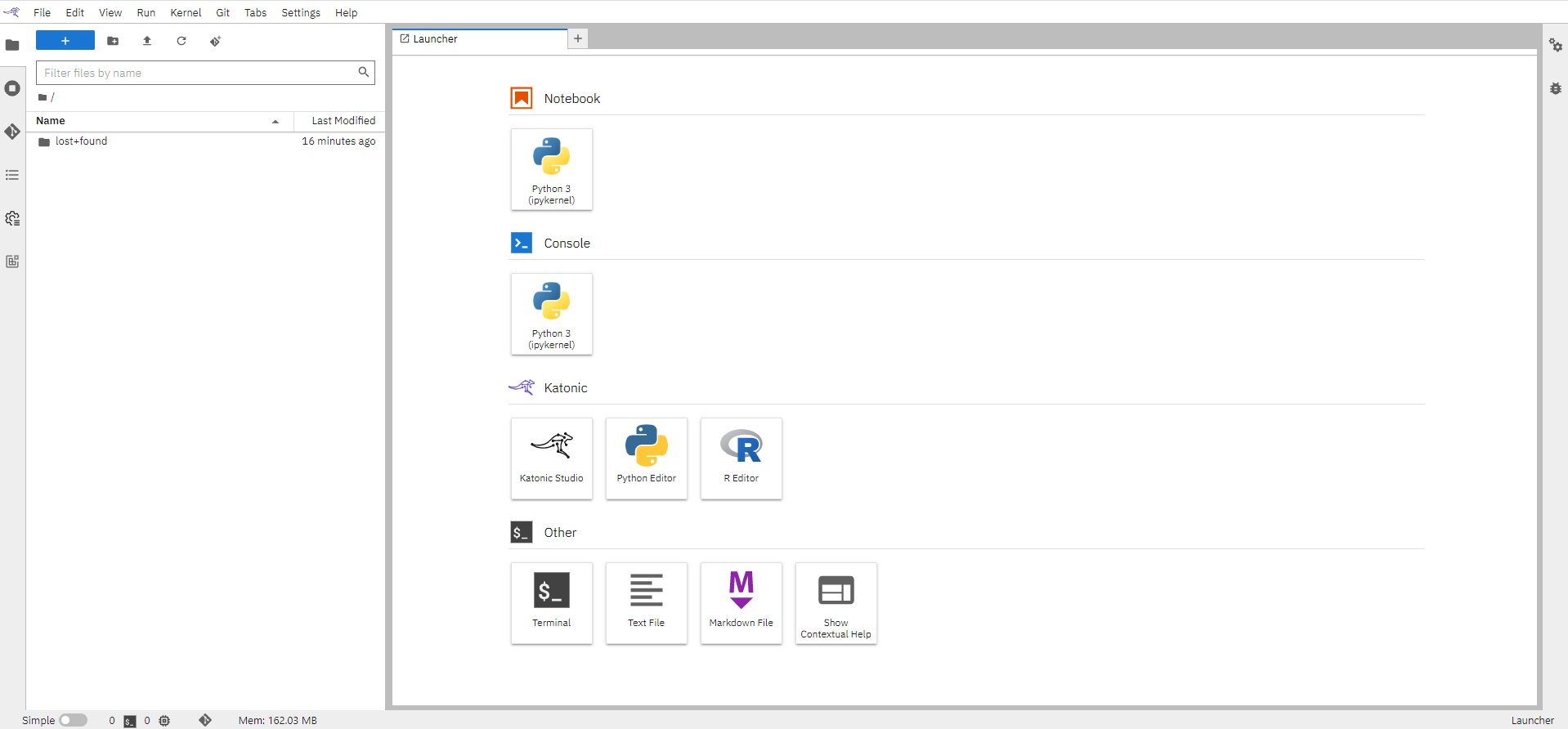
Once your notebook is up and running, you will see a fresh Jupyter interface.
If you are new to Jupyter, you might find the Jupyter documentation click here and Jupyterlab documentation click here helpful.
1.5 Configure Runtime Image
In this section, we can use the existing images or create a new custom image that will pull an already created image from your docker hub for easy access.
Click on the “Runtime Images” Icon in the left bar
Click on the “+” button on the top right
Fill in all the details on the page
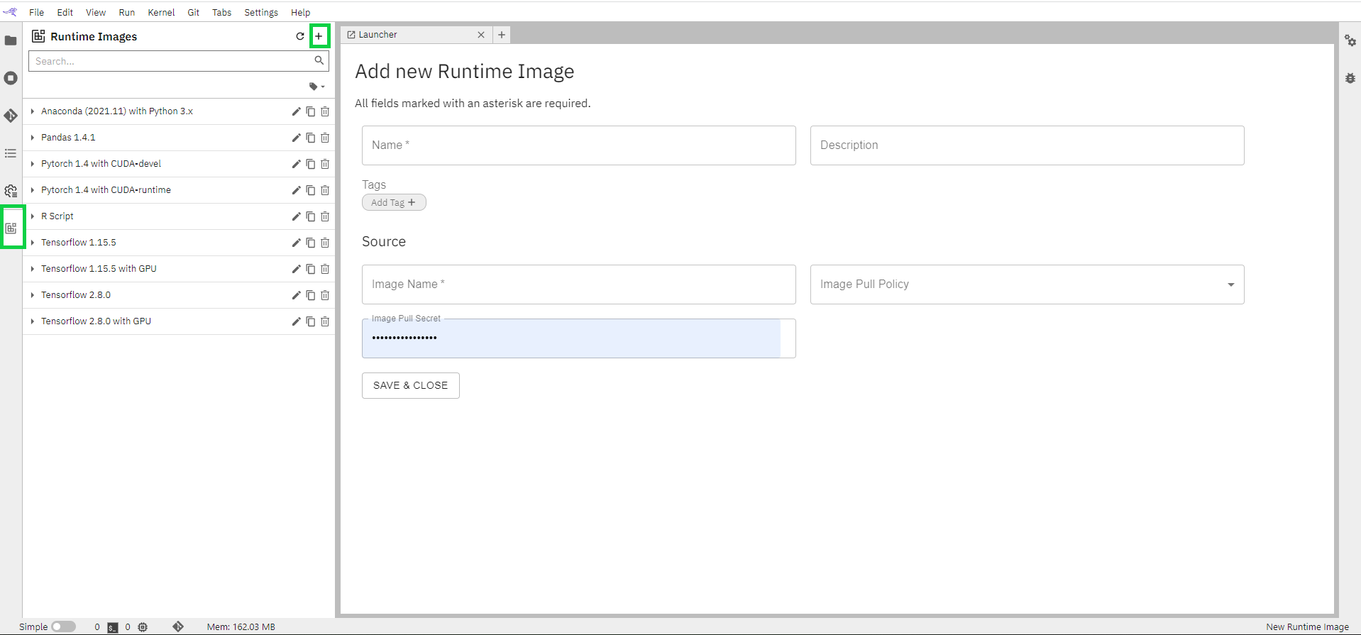
Name: User-friendly name that will appear under Runtime images list
Description(Optional) of the image. Small description defining your image
Image Name: Name of the image that you need from the docker hub.
Image Pull Policy: Select an option from the dropdown.
Click on “SAVE & CLOSE” to save the image.
A list of additional images can be seen in the left panel
1.5 Get your Files and Data
You can either upload your code and data files to your notebook space, or you can clone from Github if you maintain a repository for your codes.
If you want to perform any development activity using R language then you either use the Katonic's R-Studio Environment or Katonic's custom image katonic-R-Julia support as workspace. Follow the instructions provided in the respective documentation to access these development environments.
Once your scripts are ready on these environment, push the codes back to Github, so that they can be easily cloned to Katonic Studio workspace.
In this section, we will be showing you how can you clone data and files from our open-source R-Examples repository available on GitHub.
Click here for Katonic use cases repository specifically for examples built on R-language.
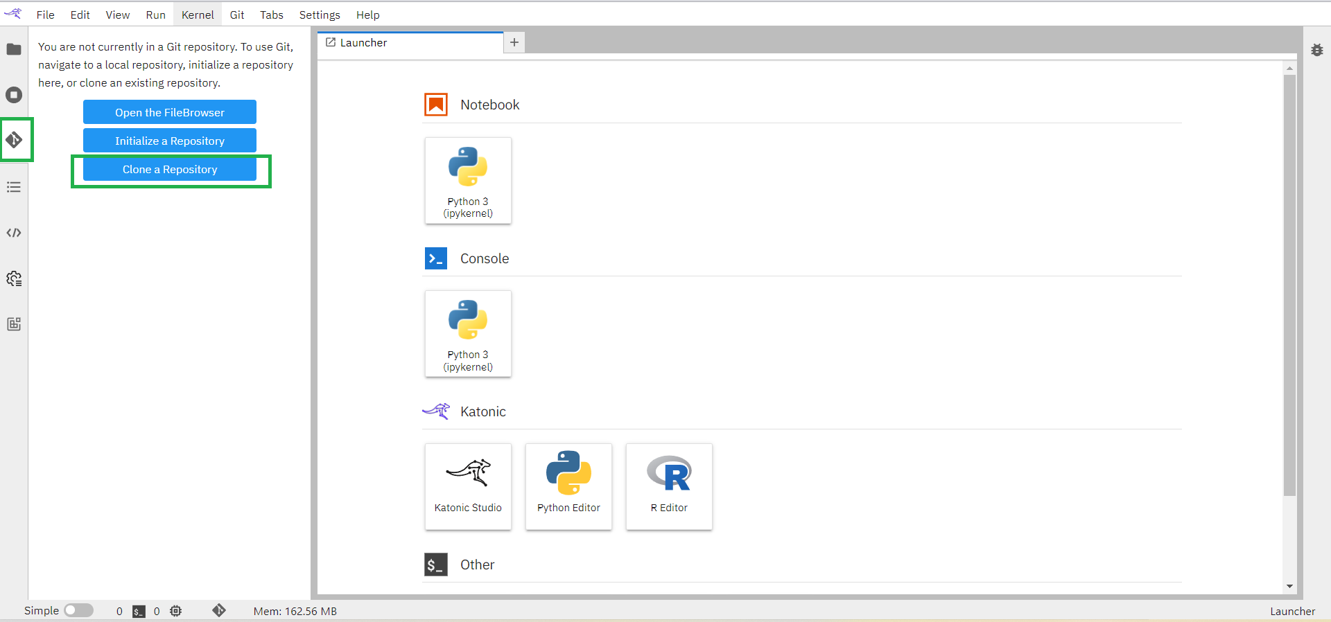
Click on the “Git” icon on the left bar
Click on the “Clone a Repository” button available in the left panel. This will open up a window.
Enter the Clone URI Link that is available in GitHub Repository.
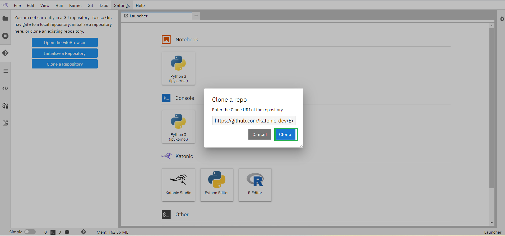
Click on the “clone” button.
This process will clone the whole repository into the workspace.
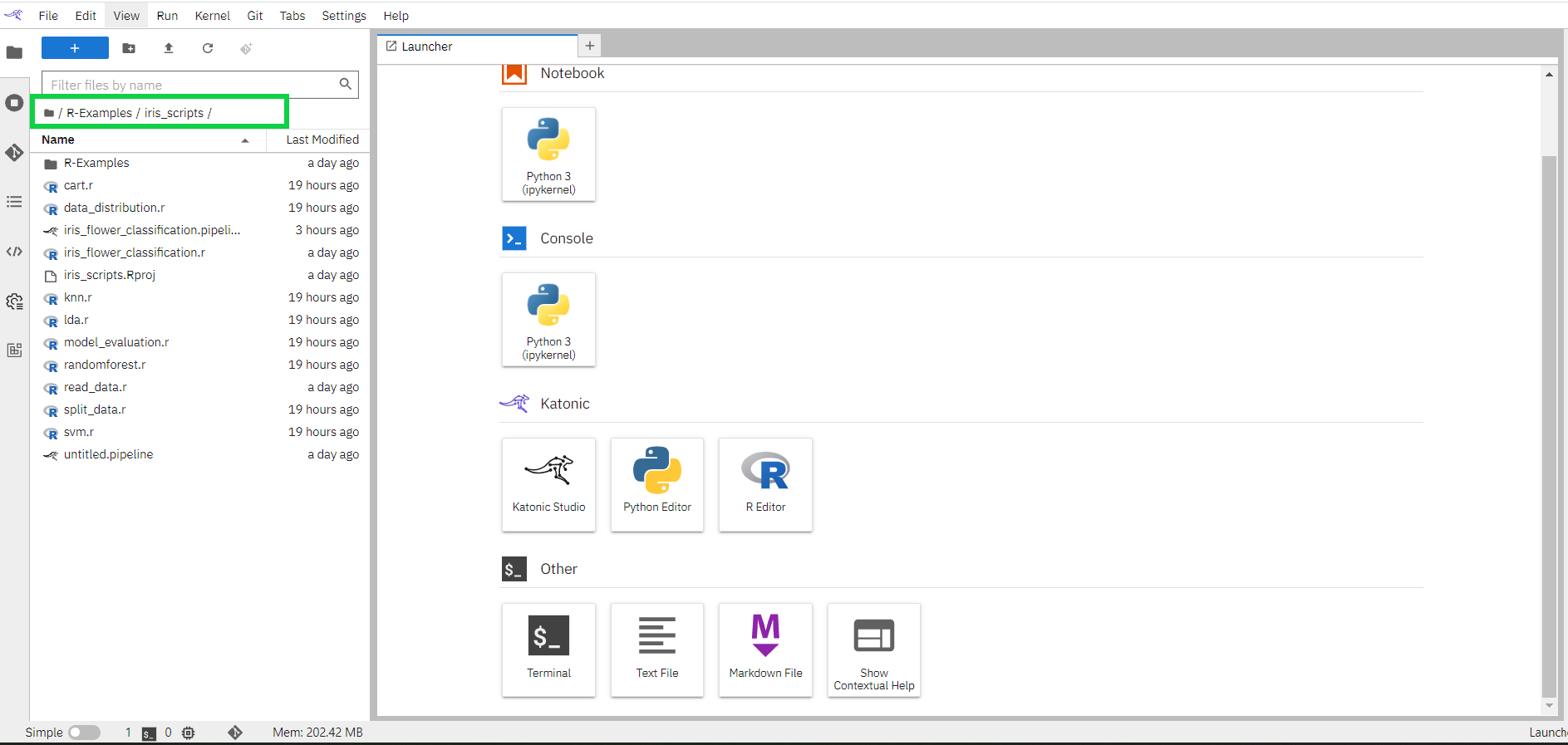
Click on “File Manager” in the left bar.
Go to location “/R-Examples/iris_scripts”.
1.7 Creating pipeline
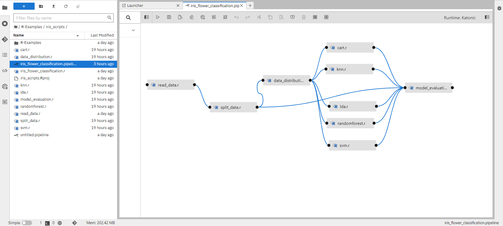
A pipeline comprises one or more nodes that are (in many cases) connected with each other to define execution dependencies. Each node is implemented by a component and typically performs only a single task, such as loading data, processing data, training a model, evaluating models or prediction.
When you open the iris_flower_classification.pipeline file it will show you the created pipeline as below.
1.7.1 How to create a pipeline component
Open the Launcher (File > New Launcher or “+” in the top left) if it is not already open.
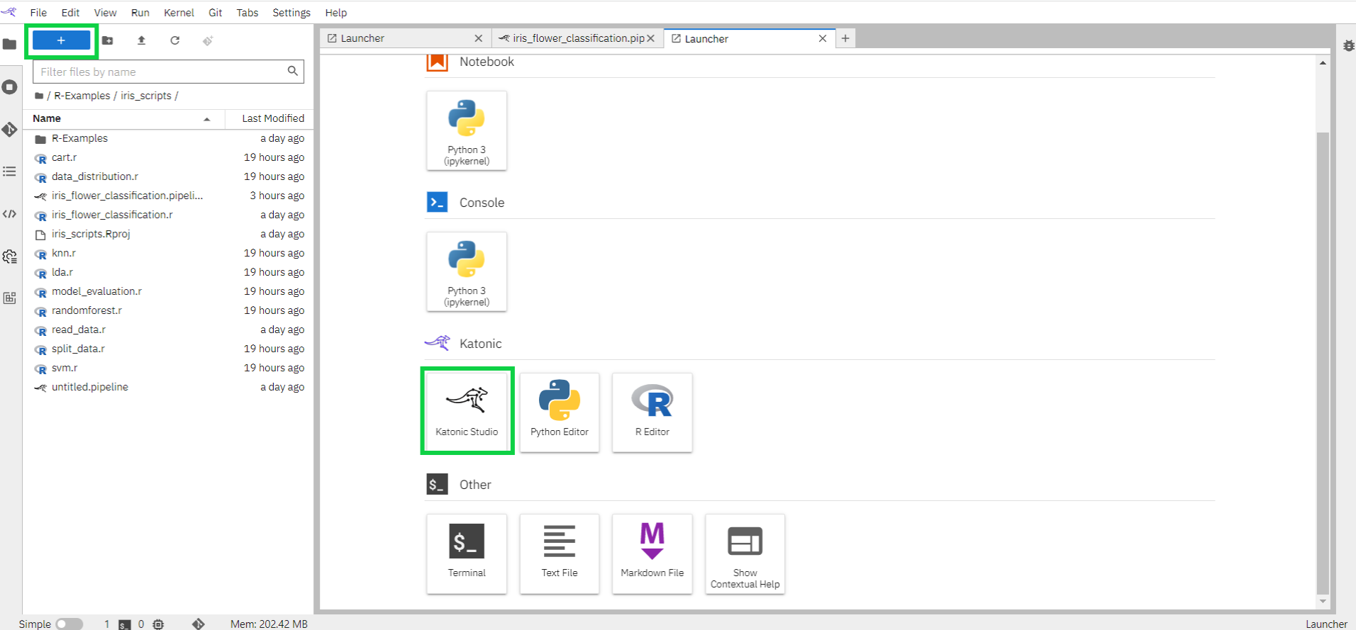
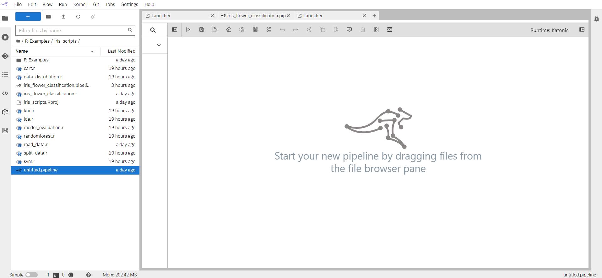
Open the pipeline editor to create a new untitled generic pipeline. Rename the pipeline to iris_flower_classification.
In the Visual Pipeline Editor open the properties panel on the right side. Select the Pipeline properties tab and fill in the pipeline details.
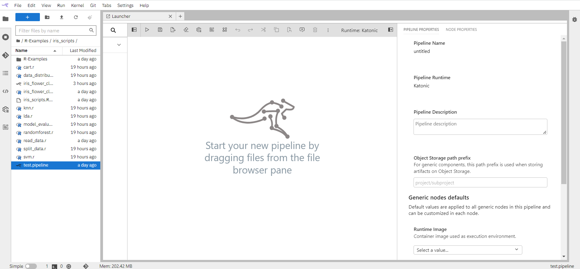
Pipeline Name: Name of the pipeline will appear here.
Pipeline Runtime: A generic pipeline comprises only of nodes that are implemented using generic components. This release includes three generic components that allow for execution of Jupyter notebooks, Python scripts, and R scripts.
Pipeline Description: An optional description summarizing the pipeline purpose.
Object Storage Path Prefix: For generic components, this path prefix is used when storing artifacts on Object Storage.
Runtime Image: As Runtime Image choose “R script”. The runtime image identifies the container image that is used to execute the notebook or R script when the pipeline is run on Kubeflow Pipelines or Apache Airflow. This setting must always be specified, but is ignored when you run the pipeline locally.
Environment Variables: If desired, you can customize additional inputs by defining environment variables.
Data volumes: Volumes to be mounted in all nodes. The specified volume Claims must exist in the Kubernetes namespace where the nodes are executed or the pipeline will not run.
Expand the component palette panel on the left-hand side. Note that there are multiple component entries, one for each supported file type.
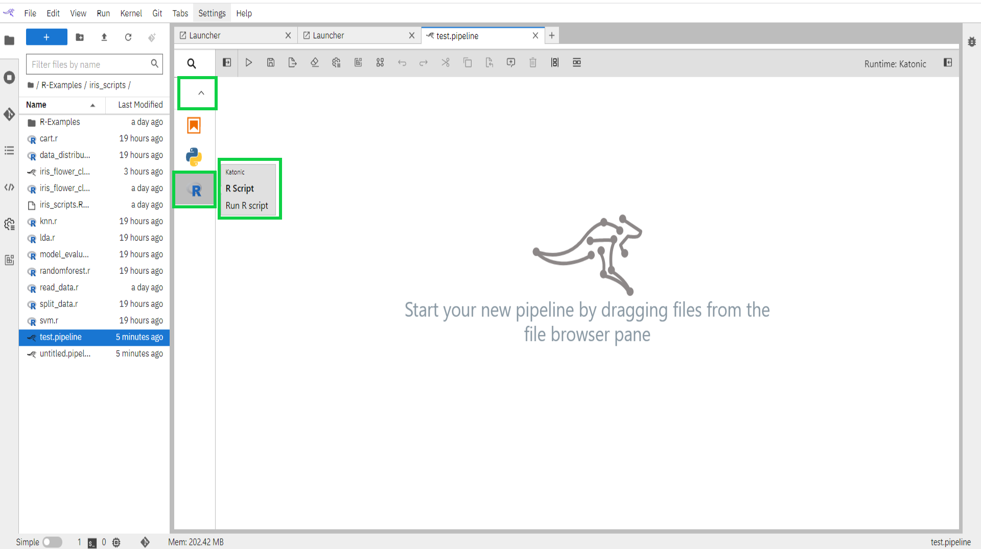
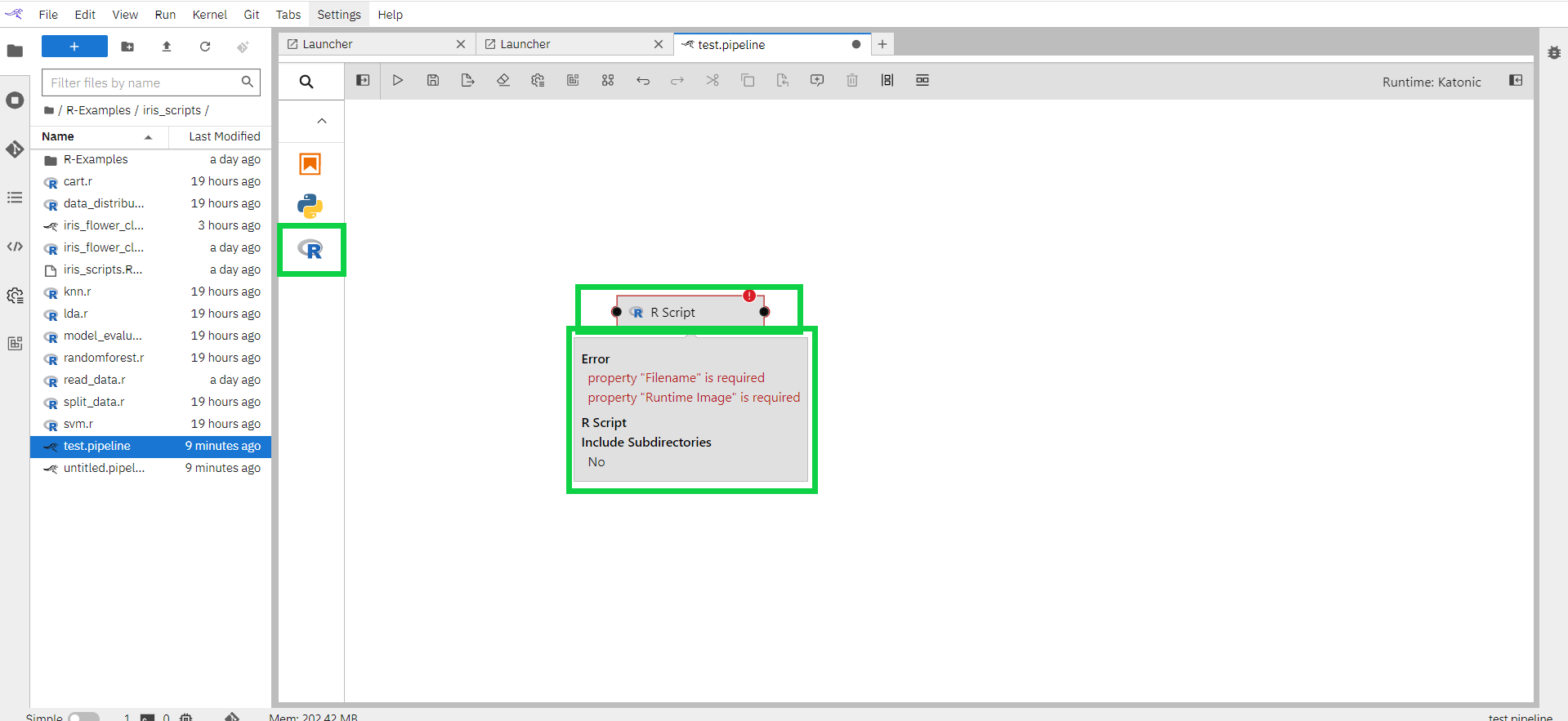
Drag the R-script component entry onto the canvas (or double click on a palette entry) and hover over the node. The error messages are indicating that the node is not yet configured properly.
Select the newly added node on the canvas, right-click, and select Open Properties from the context menu.
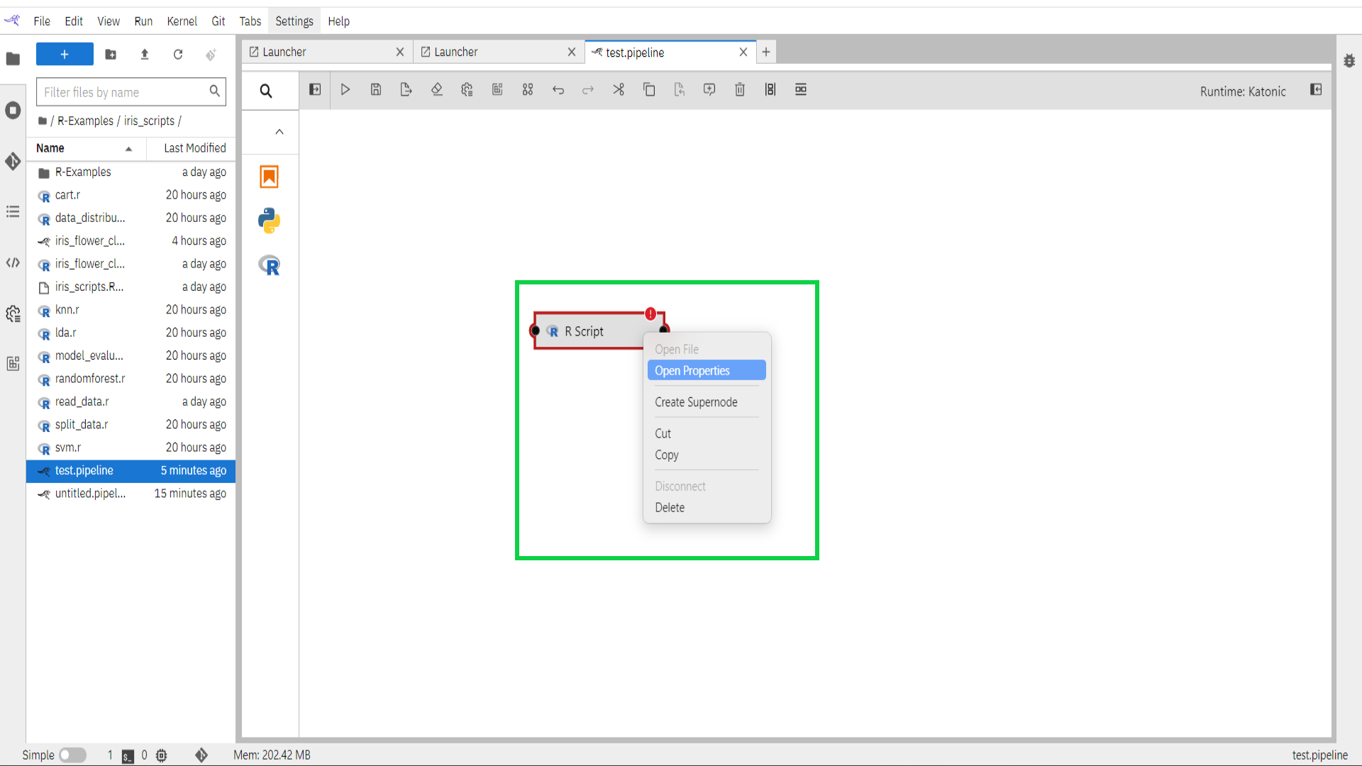
Configure the node properties.
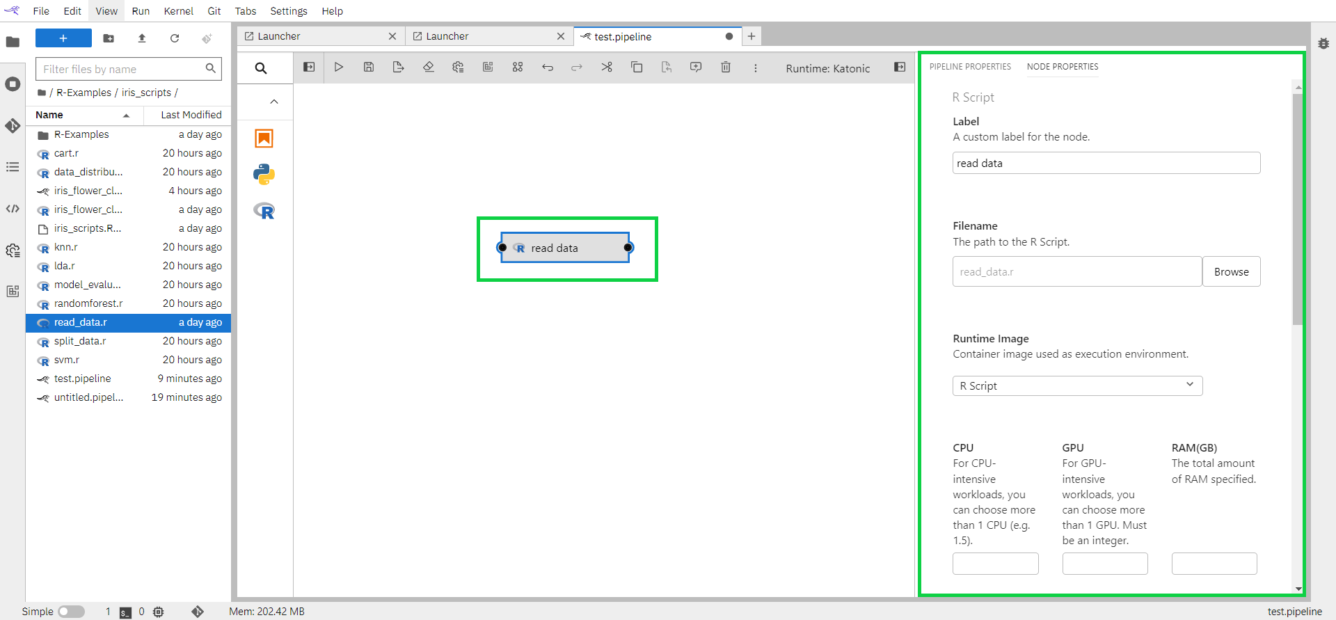
Label: Assign the node a descriptive label. If you leave the label empty, the file name will be used.
Filename: Browse to the file location. Navigate to the “/R-Examples/iris_scripts” directory and select “read_data.r”.
Runtime Image: As Runtime Image choose “quay.io/katonic/common:r-base”. This image will not be available in the dropdown. Follow the instructions from section 1.6 Configure Runtime Image above to add this image. Once the image is added you can refresh the page and this image name would appear in the dropdown.
The runtime image identifies the container image that is used to execute the notebook or R script when the pipeline is run on Kubeflow Pipelines. This setting must always be specified but is ignored when you run the pipeline locally.CPU/GPU/RAM: If the container requires a specific minimum amount of resources during execution, you can specify them.
File Dependencies: The read_data file does not have any input file dependencies. Leave the input field empty.
Environment Variables: If desired, you can customize additional inputs by defining environment variables.
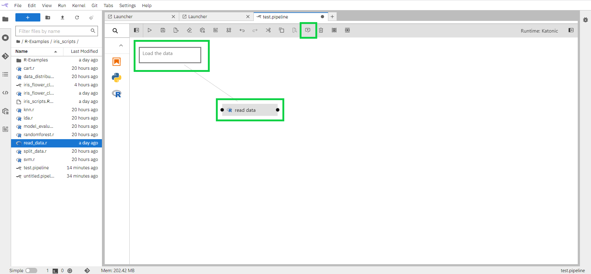
For a component, you can comment from the comment button.
Select the component
Click on the comment button on the top
1.7.2 How to connect components
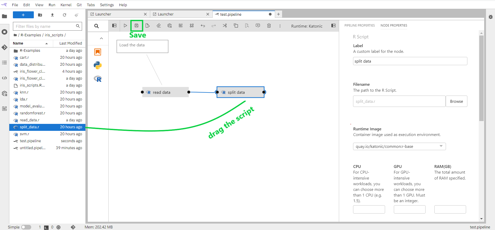
Earlier in this tutorial, you added a (R script) file component to the canvas using the palette. You can also add Jupyter notebooks, Python scripts to the canvas by dragging and dropping from the JupyterLab File Browser.
From the JupyterLab File Browser drag and drop the “split data.r” notebook from location “/R-Examples/iris_scripts“ onto the canvas.
Customize the file's execution properties as follows:
Runtime image: quay.io/katonic/common:r-base
Output files: train.csv and validation.csv
Connect the output port of the read_data node to the input port of the split_data node to establish a dependency between the two scripts.
Save the pipeline.
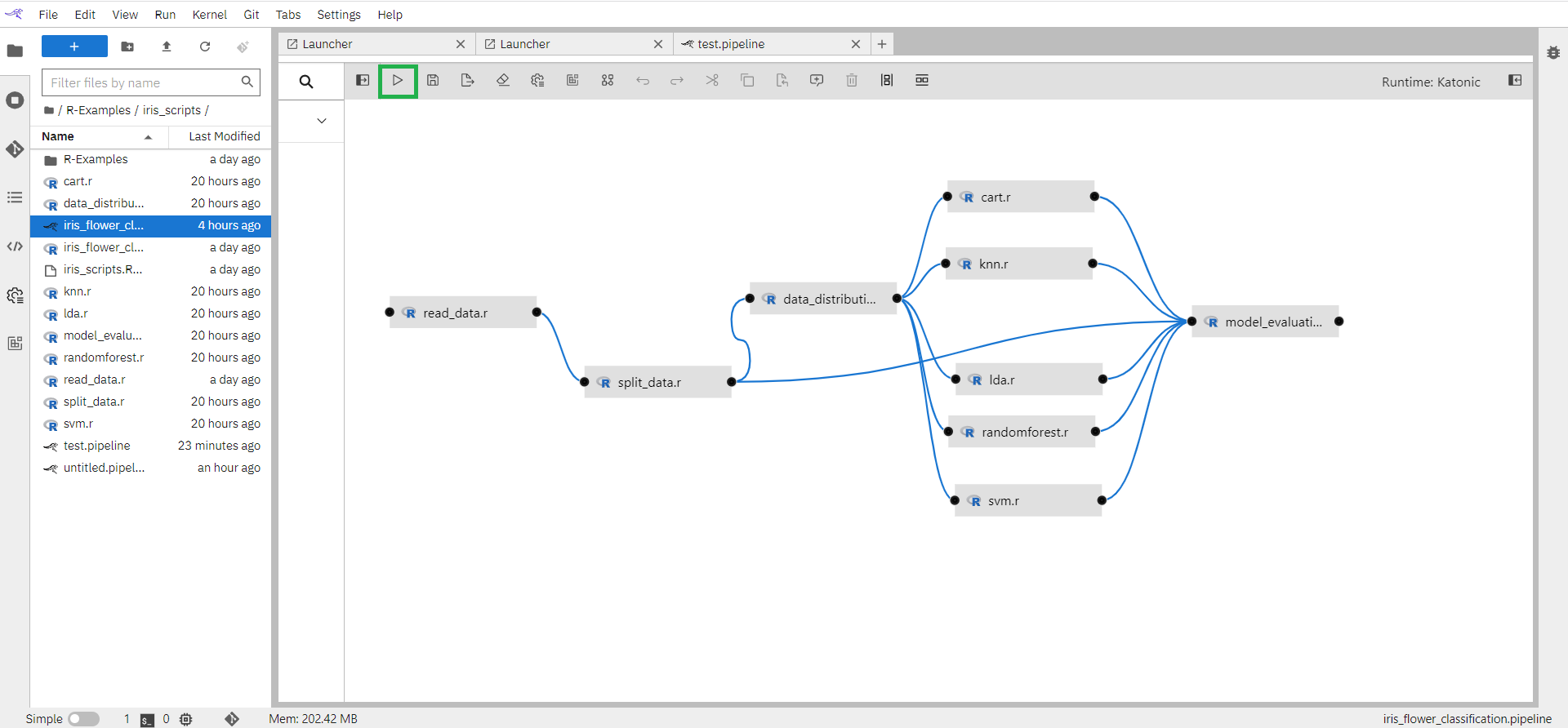
1.7.3 Iris Flower Classification Pipeline Flow
Earlier in the tutorial, we have how to create pipeline components and connect the components. In this section, we will see how the end-to-end iris flower classification pipeline is implemented.
Open "iris_flower_classification.pipeline” pre-build pipeline for iris flower classification use case.
When you double click on any of the components it will open the R script file.
In every component, you should read the output from the previous step and save the results of the current step.
Read Data: Read the iris dataset already available in R. Save the result in the iris.csv file
# attach the iris dataset to the environment
data(iris)

# rename the dataset
dataset <- iris

colnames(dataset) <- c("Sepal.Length","Sepal.Width","Petal.Length","Petal.Width","Species")

write.csv(dataset,'iris.csv',row.names = FALSE)
- Split Data: It reads the outfile file of read data script and after processing saves the results in train.csv and validation.csv files.
install.packages("caret", dependencies=c("Depends", "Suggests"),repos = "http://cran.us.r-project.org")

install.packages("gower",repos = "http://cran.us.r-project.org")
install.packages("parallelly",repos = "http://cran.us.r-project.org")
install.packages("ModelMetrics",repos = "http://cran.us.r-project.org")
library(caret)

dataset<-read.csv("iris.csv")

# create a list of 80% of the rows in the original dataset we can use for training
validation_index <- createDataPartition(dataset$Species, p=0.80, list=FALSE)
# select 20% of the data for validation
validation <- dataset[-validation_index,]
# use the remaining 80% of data to training and testing the models
dataset <- dataset[validation_index,]

# dimensions of dataset
dim(dataset)

sapply(dataset, class)

head(dataset)
head(validation)

percentage <- prop.table(table(dataset$Species)) * 100
cbind(freq=table(dataset$Species), percentage=percentage)

# summarize attribute distributions
summary(dataset)

write.csv(dataset,'train.csv',row.names=FALSE)
write.csv(validation,'validation.csv',row.names=FALSE)
Similarly, other scripts also follows the same structure of reading the output file of previous scripts and saving the output of for downstream files.
Now pipeline is built and ready. Save the pipeline to run.
1.8 Run Pipeline
In the previous section, we have seen how the generic pipeline and iris flower classification pipeline is built. In this section, you will learn how to run a pipeline in the Kubeflow runtime environment.
Run pipeline from the button available on the top bar.
Enter pipeline name (eg: iris flower classification), select Runtime Platform as Kubeflow Runtime, and click on the “OK” button.
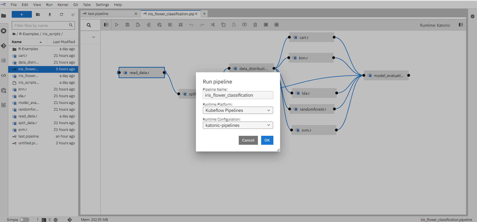
Pipeline is now submitted to Kubeflow environment. Click on “OK”.
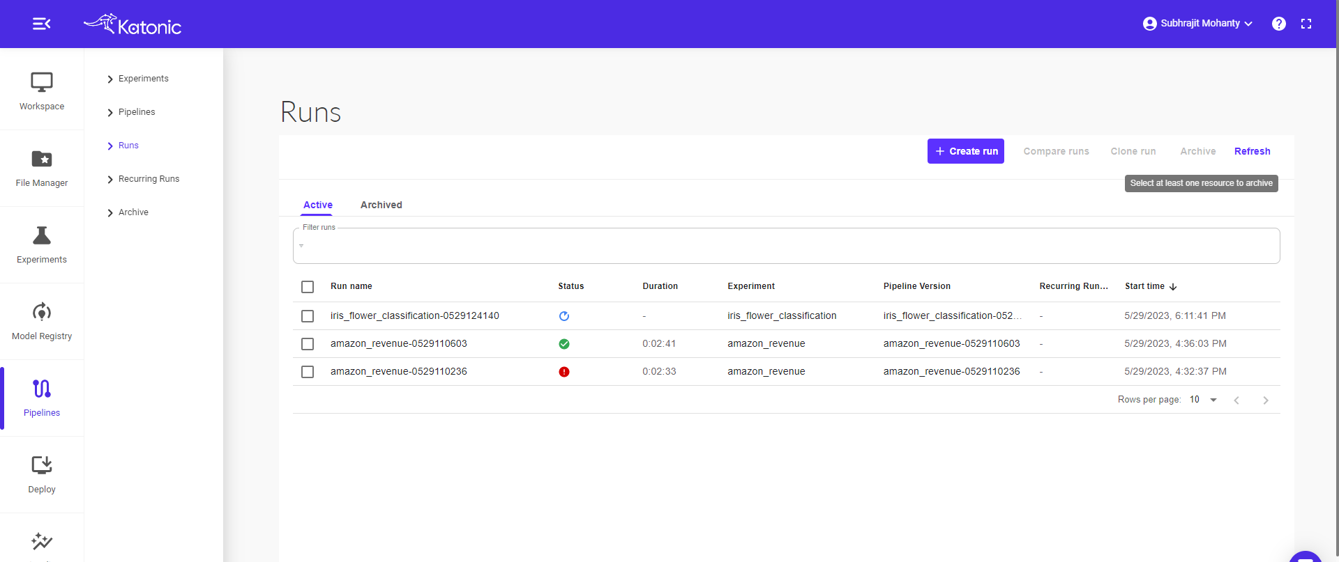
The pipeline will run in the Kubeflow environment. You can see the pipeline in Pipeline section of the left panel of the platform.

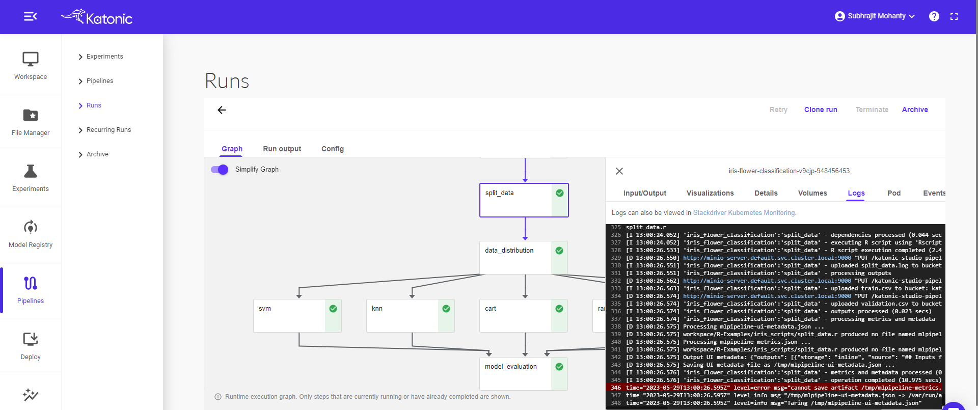
Click on the pipeline to view the complete pipeline. The pipeline status is in Running stage. Once all the components ran successfully it will show a green tick on every component.
Note: To view the pipeline clearly use “full screen mode" (button available on the top right).
Click on the component to see the logs and visualizations of the current step.
1.9 Schedule Pipeline
In the previous section, we have seen how to run the Kubeflow pipeline. In this section, you will learn how to schedule this pipeline or re-run the same pipeline again.
Go to Pipeline section and select Runs in the left sidebar.
Click on “Create Run” to run the pipeline or schedule the pipeline.
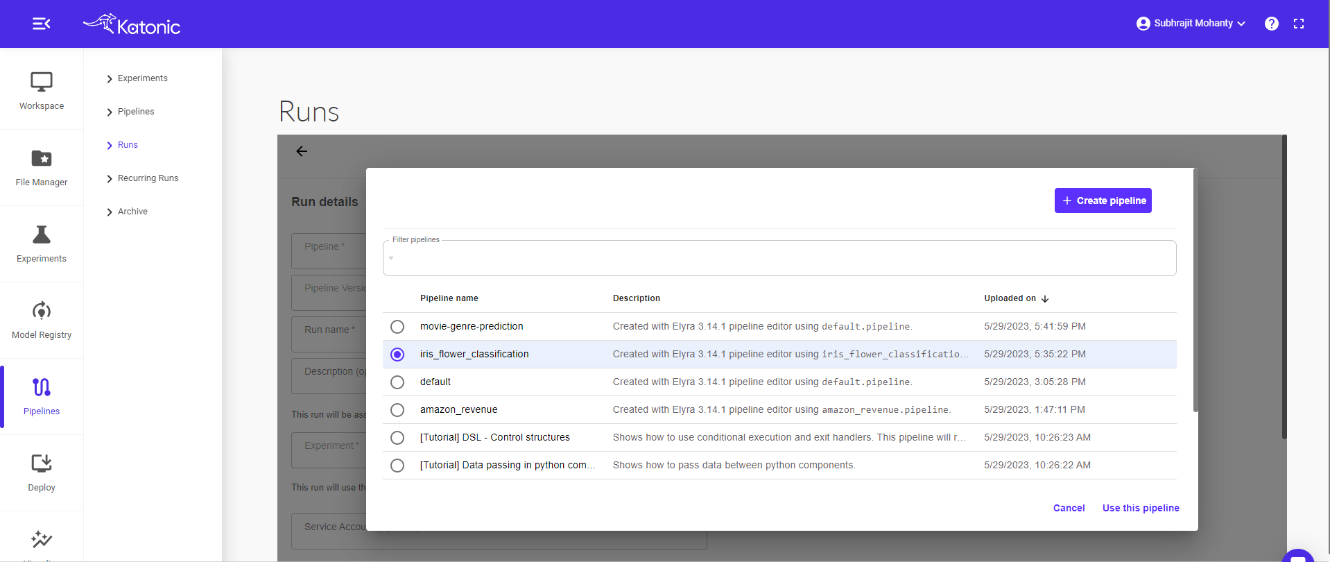
Click on Choose in the pipeline text box.
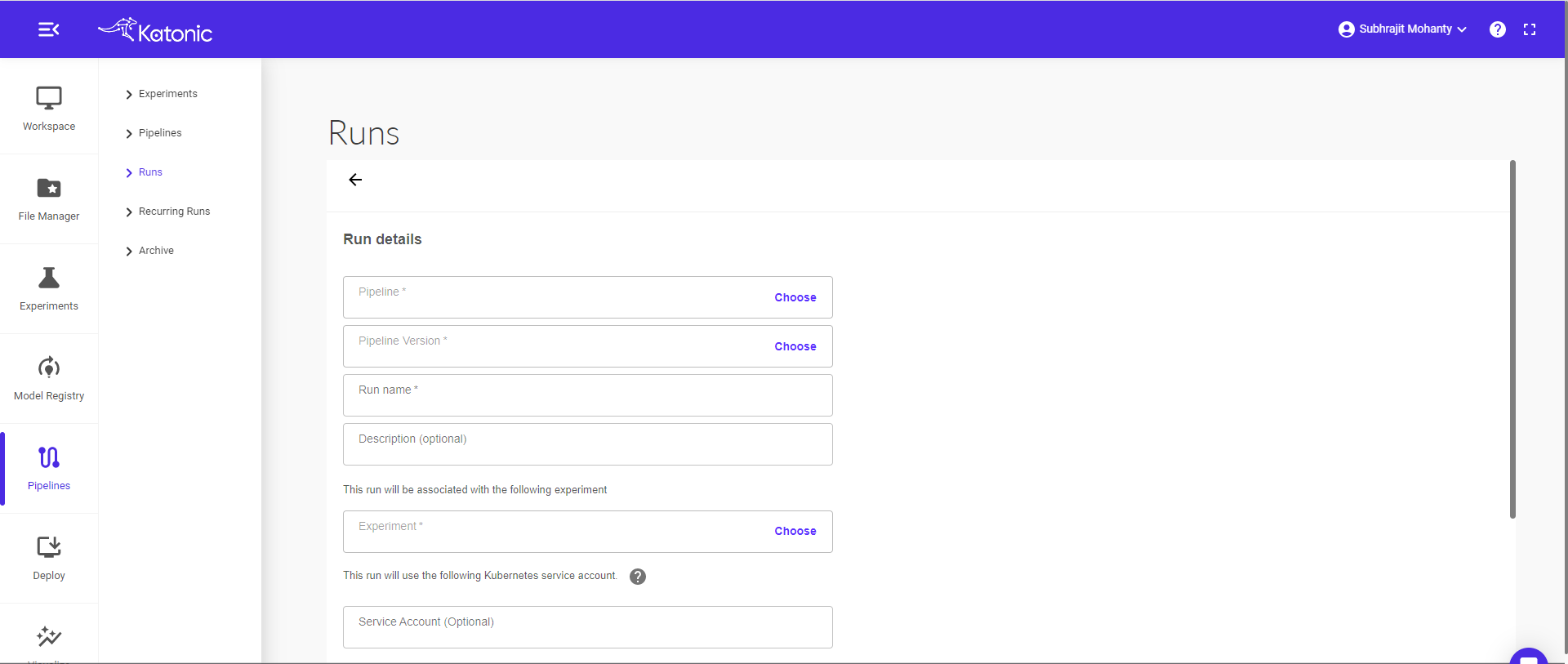
Select a pipeline that you want to run or schedule (Eg: iris flower classification). Click on the “Use this pipeline” button.
Give a new Run Name (Eg: iris_flower_classification_scheduling). Also choose the respective experiment name under which you want to perform your run.
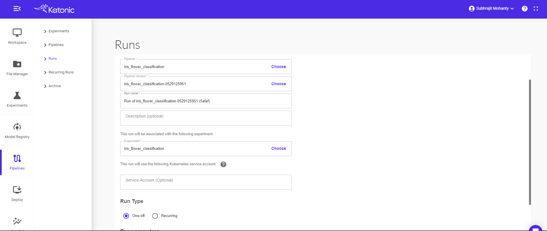
The pipeline can be run in two ways i.e., run once or schedule
Run Once: Select Run Type as One-off radio button and click on start to run the pipeline.
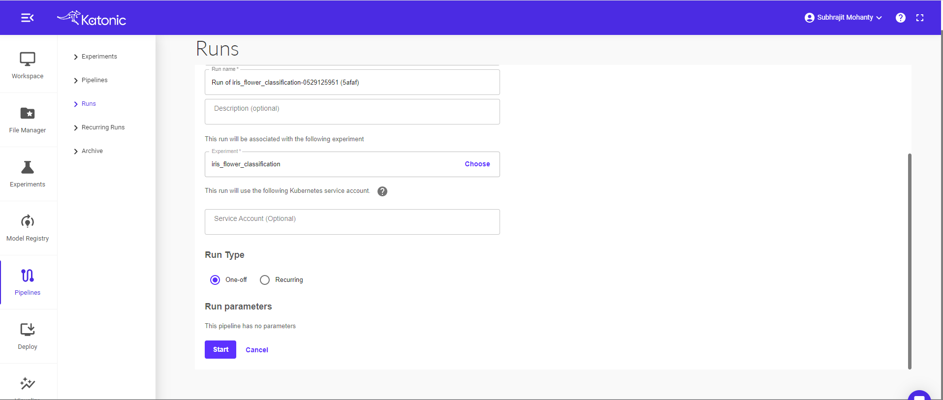
Scheduling: Select Run Type as Recurring.

- Trigger Type: Select if the pipeline should run as a Periodic or cron Job.
- Maximum Concurrent Runs: limit the number of runs launched in parallel
- Start Date and End Date: Give the start and end date of the scheduler (Optional)
- Catchup: Specify how many runs every minute/hour/day/week/month.
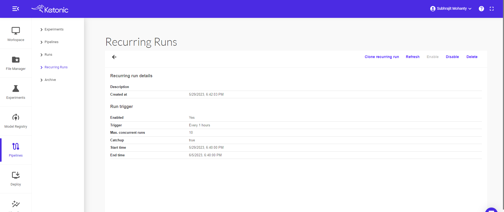
Scheduled runs can be seen here in the Recurring Runs.
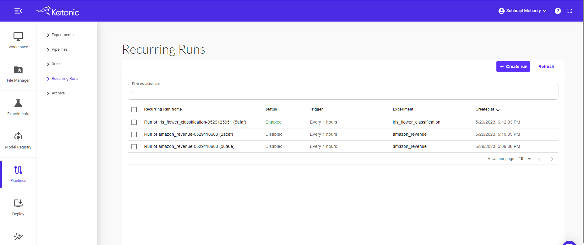
Click on run to check the schedule configurations.